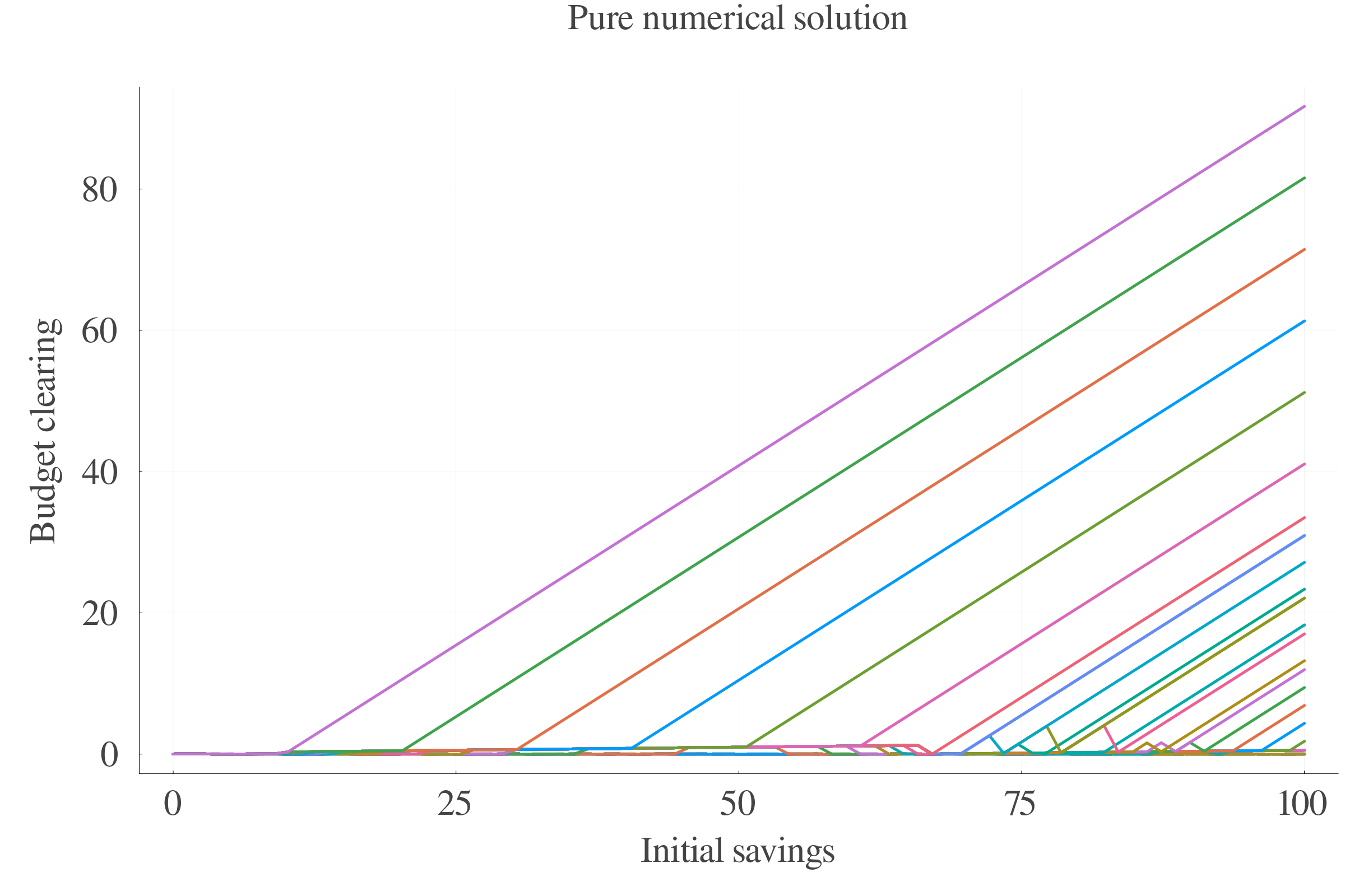
Analytical solution inexistence
\[ \max_{\{c_{t},l_{t},s_{t+1}\}_{t=1}^{100}}
{\mathbb{E}\left[\sum_{t=1}^{100} \beta^{t}\cdot \frac{c_{t}^{1-\rho}}{1-\rho}-\xi_{t}\cdot \frac{l_{t}^{1+\varphi}}{1+\varphi}\right]}\]
Subject to budget and borrowing constraints:
\[c_{t} + s_{t+1} \leq l_{t}\cdot z_{t} + s_{t}\cdot(1+r_{t})\]
\[s_{t+1}\geq \underline{s}, \forall t \in [\![1,100]\!]\]
A first solving attempt consists in assuming that the budget constraint binds. We can then obtain the following expression for consumption:
\[c_{t} = l_{t}\cdot z_{t} + s_{t}\cdot(1+r_{t}) - s_{t+1}\]
Plugging it into the maximization program, we obtain:
\[ \max_{\{l_{t},s_{t+1}\}_{t=1}^{100}}
{\mathbb{E}\left[\sum_{t=1}^{100} \beta^{t}\cdot \frac{\left(l_{t}\cdot z_{t} + s_{t}\cdot(1+r_{t}) - s_{t+1}\right)^{1-\rho}}{1-\rho}-\xi_{t}\cdot \frac{l_{t}^{1+\varphi}}{1+\varphi}\right]}\]
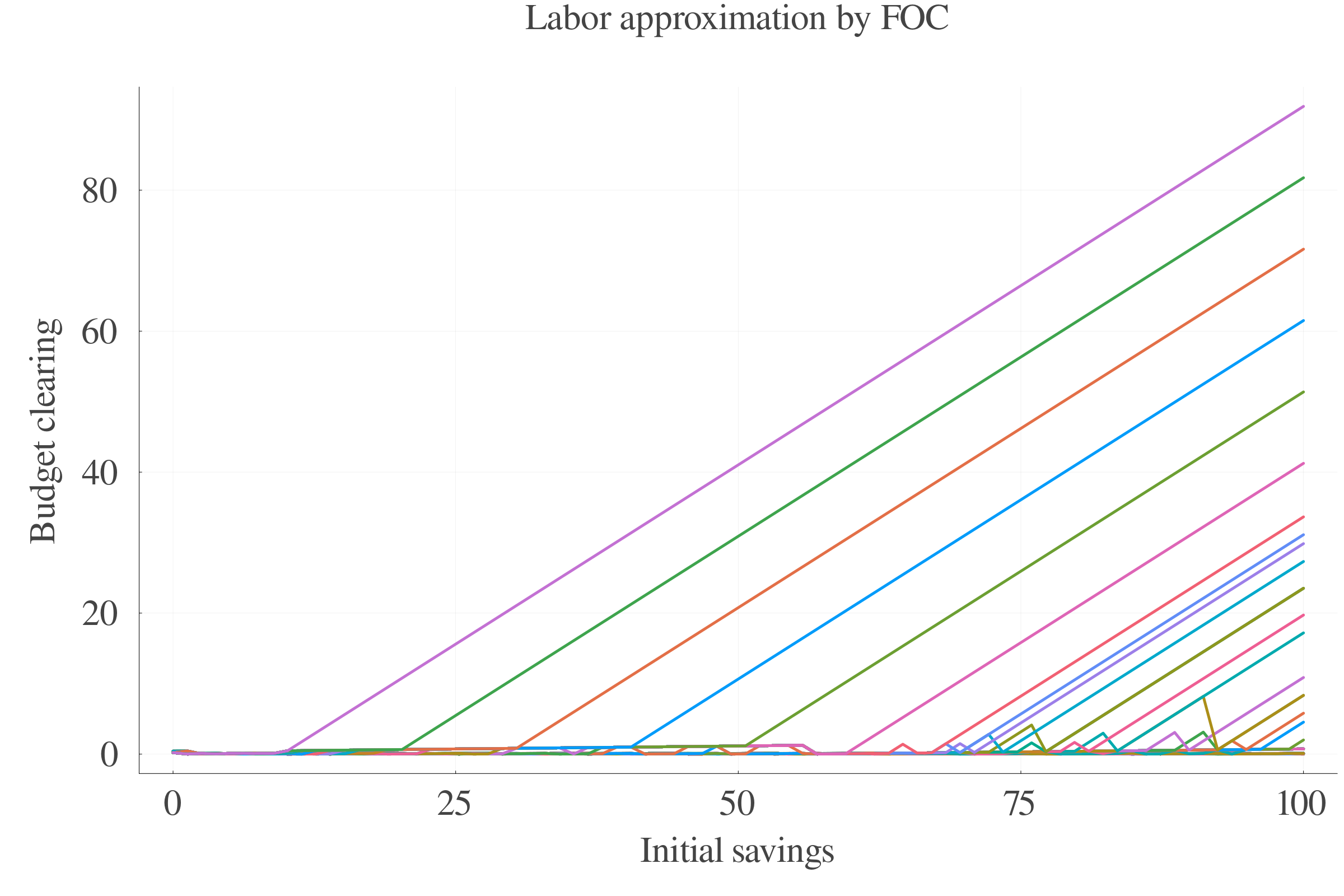
The F.O.C. with respect to labor implies:
\[\begin{equation}
l_{t}^{\varphi}\cdot \xi_{t} = \left[l_{t}\cdot z_{t} + s_{t}\cdot(1+r_{t})- s_{t+1}\right]^{-\rho}\cdot z_{t}
\end{equation}\]
We can develop the decomposition of consumption if and only if \(\rho \in \mathbb{N}\). Indeed, this equation is of form \(x = (x-\alpha)^{\beta} \cdot z\). With \(\beta\notin \mathbb{N}\), is a transcendental equation.
We can now try to compute the F.O.C. first, and then make use of the Budget Constraint. The Lagrangian function associated witht the maximization program of the agent is: \[\begin{equation}
\begin{split}
\mathcal{L}(c_{t},l_{t},s_{t+1};\lambda_t,\gamma_{t}) &
= \mathbb{E}\Big[\sum_{t=1}^{100} \beta^{t}\cdot ((\frac{c_{t}^{1-\rho}}{1-\rho}-\xi_{t}\cdot\frac{l_{t}^{1+\varphi}}{1+\varphi}) \\
& +\lambda_{t}\cdot \left(l_{t}\cdot z_{t}+s_{t}\cdot (1+r_{t})-c_{t}-s_{t+1}\right) \\
& + \gamma_{t}\cdot \left(s_{t+1}-\underline{s}\right))\Big] \\
\end{split}
\end{equation}\]
The First Order Conditions are the following:
\[\frac{\partial \mathcal{L}}{\partial c_{t}} = 0 \iff c_{t}^{-\rho} = \lambda_{t}\]
\[\frac{\partial \mathcal{L}}{\partial l_{t}} = 0 \iff \lambda_{t}\cdot z_{t} = \xi_{t}\cdot l_{t}^{\varphi}\]
\[\frac{\partial \mathcal{L}}{\partial s_{t+1}} = 0 \iff \lambda_{t} = \beta \cdot \mathbb{E}\left[\lambda_{t+1}\cdot (1+r_{t+1})\right] + \gamma_{t}\]
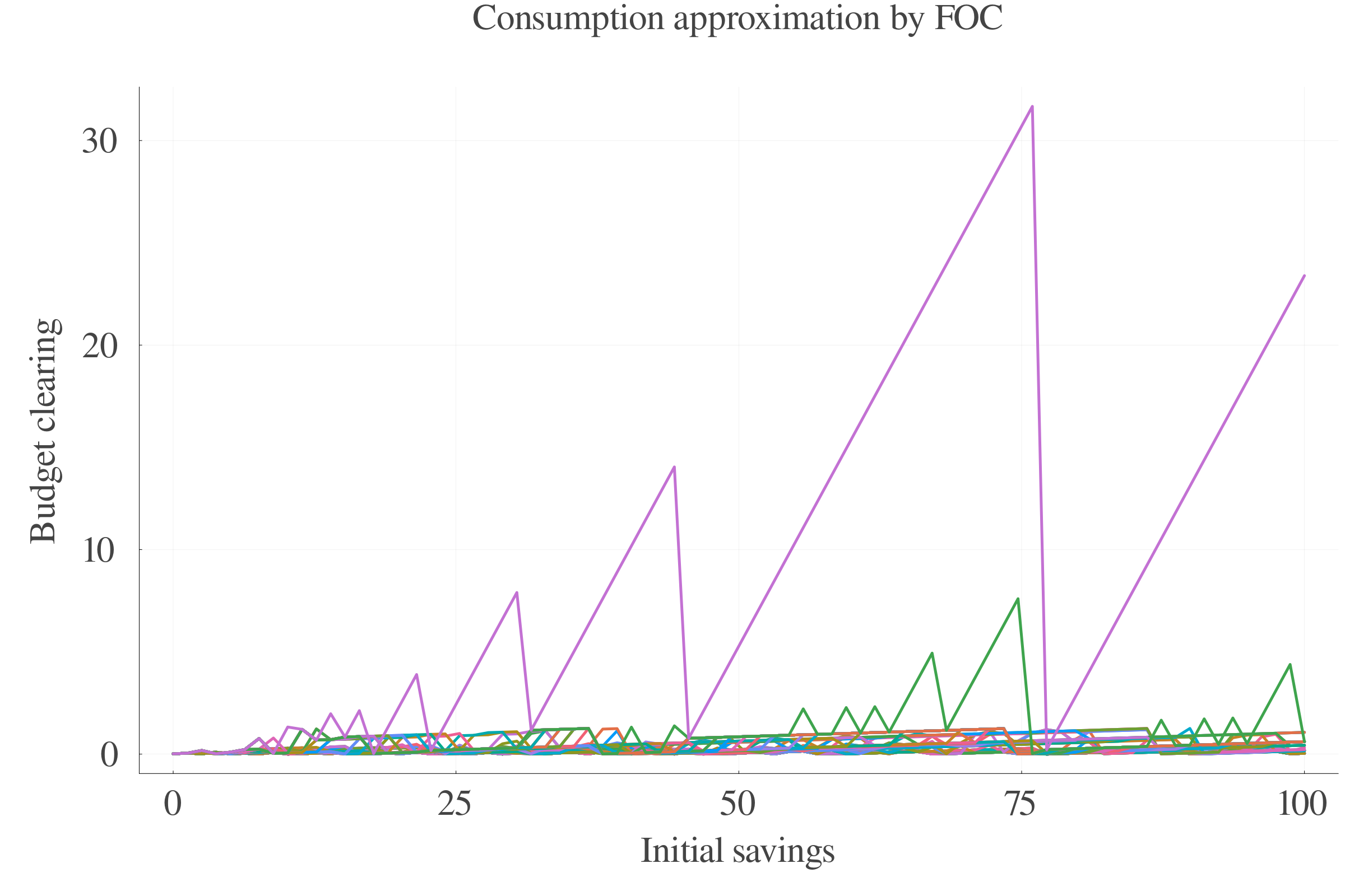
We first note that we must obtain a closed-form solution for \(c_{t}\) and \(l_{t}\) to obtain the optimal value of \(s_{t+1}\). Indeed, since \(s_{t+1}\) is linear in \(\mathcal{L}\), we would need to plug the closed-form solutions of \(c_{t}\) and \(l_{t}\) in the budget constraint.
Replacing the expression of \(\lambda_{t}\) in the two other equation yields:
\[\begin{equation}
c^{-\rho}_{t}\cdot z_{t} = \xi_{t}\cdot l_{t}^{\varphi} \iff
\begin{cases}
& c_t = \left[\frac{\xi_{t}\cdot l_{t}^{\varphi}}{z_{t}}\right]^{-\frac{1}{\rho}}\\
& l_{t} = \left[\frac{c_{t}^{-\rho}z_{t}\cdot}{\xi_{t}}\right]^{\frac{1}{\varphi}}
\end{cases}
\end{equation}\] And \[\begin{equation}
c^{-\rho}_{t} = \beta \cdot \mathbb{E}\left[c^{-\rho}_{t+1}\cdot (1+r_{t+1})\right] + \gamma_{t}
\end{equation}\]
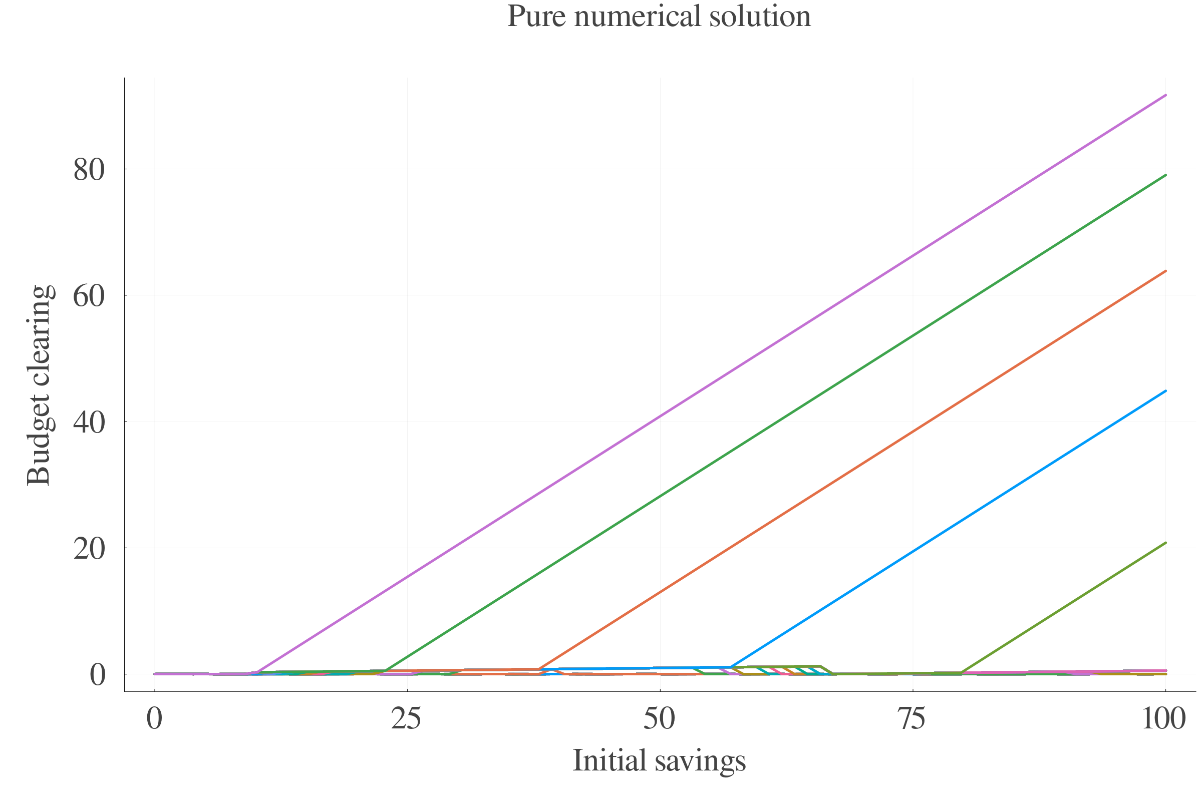
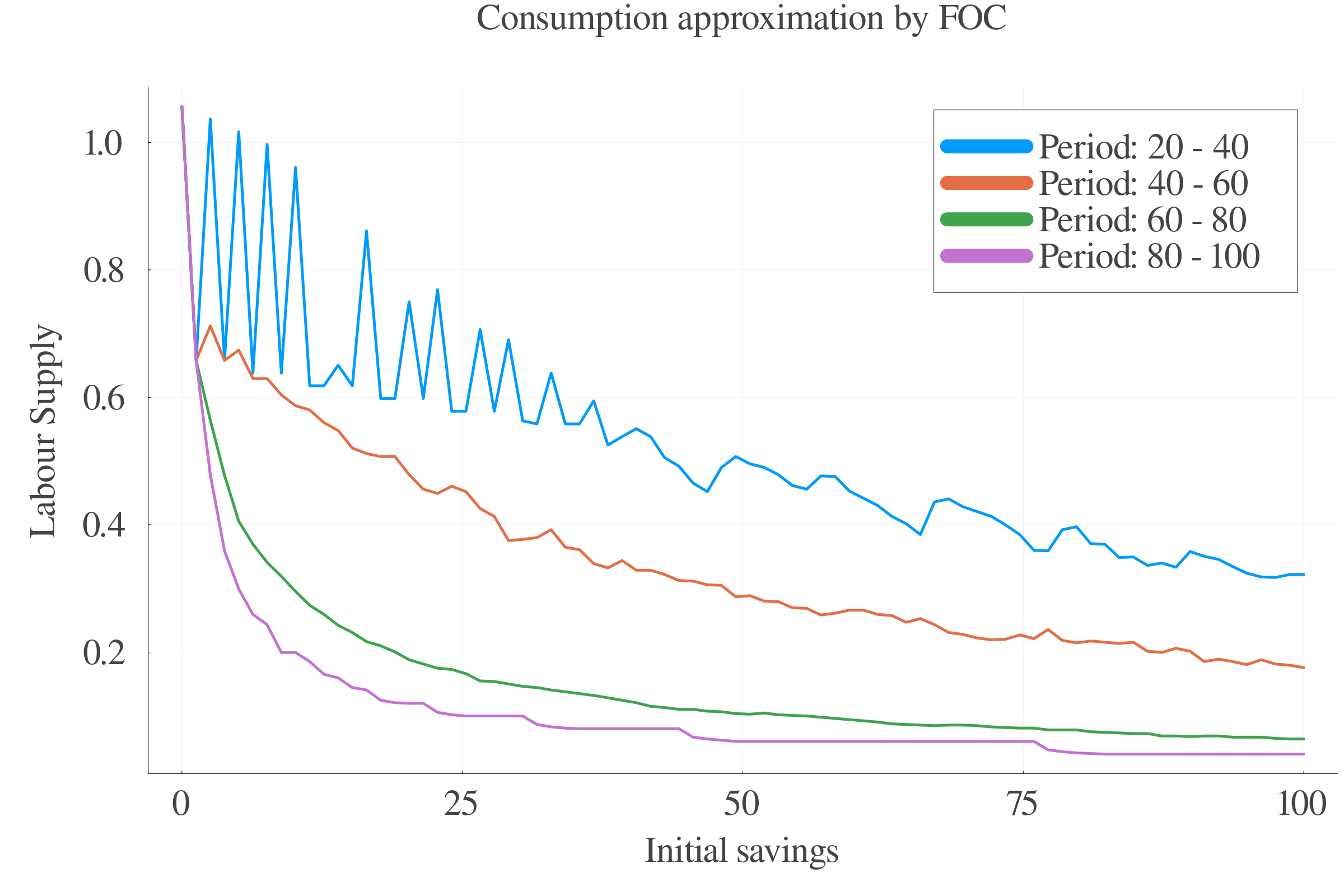
Assuming that the budget constraint binds, it becomes, as previously seen:
\[c_{t} + s_{t+1} = l_{t}\cdot z_{t} + s_{t}\cdot(1+r_{t})
\iff
c_{t} = l_{t}\cdot z_{t} + s_{t}\cdot(1+r_{t}) - s_{t+1}
\]
This leads to the following equation system:
\[
\begin{cases}
& c_t = \left[\frac{\xi_{t}\cdot l_{t}^{\varphi}}{z_{t}}\right]^{-\frac{1}{\rho}} \\
& c_{t} = l_{t}\cdot z_{t} + s_{t}\cdot(1+r_{t}) - s_{t+1}
\end{cases}
\]
\[\iff\] \[ \left[\frac{\xi_{t}\cdot l_{t}^{\varphi}}{z_{t}}\right]^{-\frac{1}{\rho}} = l_{t}\cdot z_{t} + s_{t}\cdot(1+r_{t}) - s_{t+1} \] \[\iff\] \[ l_{t}^{-\frac{\varphi}{\rho}} \cdot \left(\frac{\xi_{t}}{z_{t}}\right)^{-\frac{1}{\rho}} = l_{t}\cdot z_{t} + s_{t}\cdot(1+r_{t}) - s_{t+1} \] \[\iff\] \[ l_{t}^{-\frac{\varphi}{\rho}} \cdot \left(\frac{z_{t}}{\xi_{t}}\right)^{\frac{1}{\rho}} - l_{t}\cdot z_{t} - s_{t}\cdot(1+r_{t}) - s_{t+1} = 0 \]
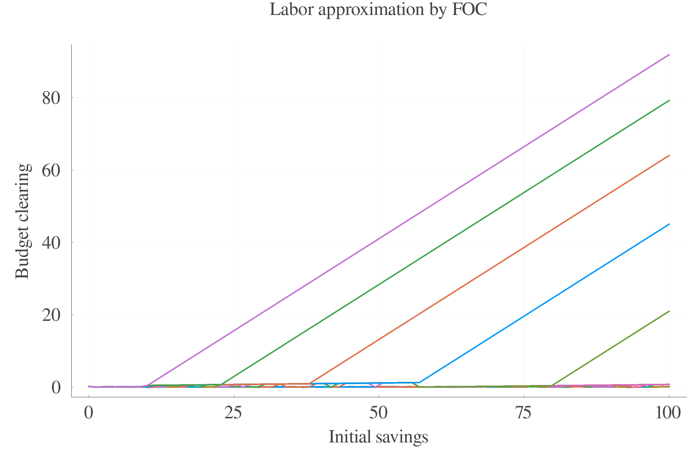
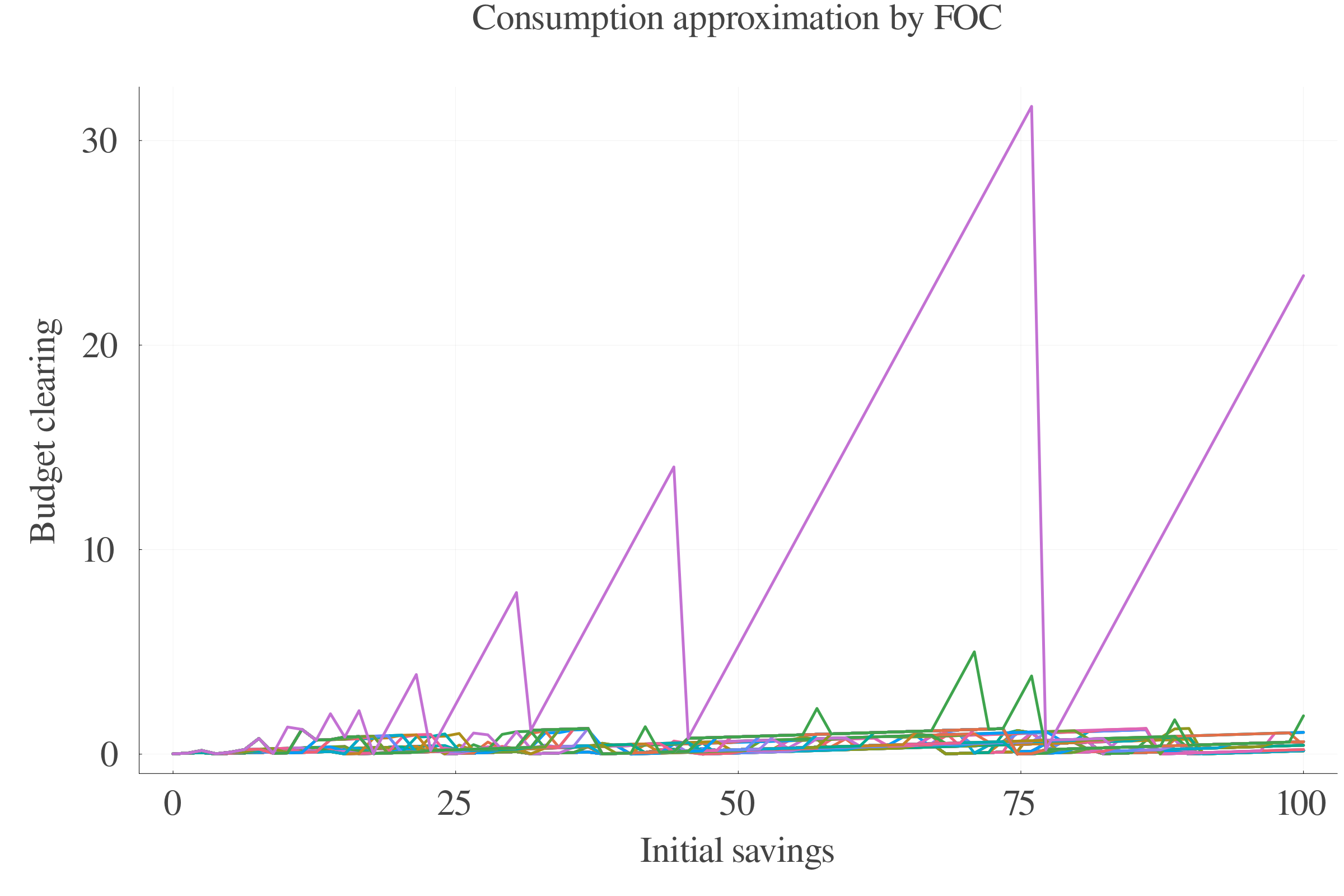
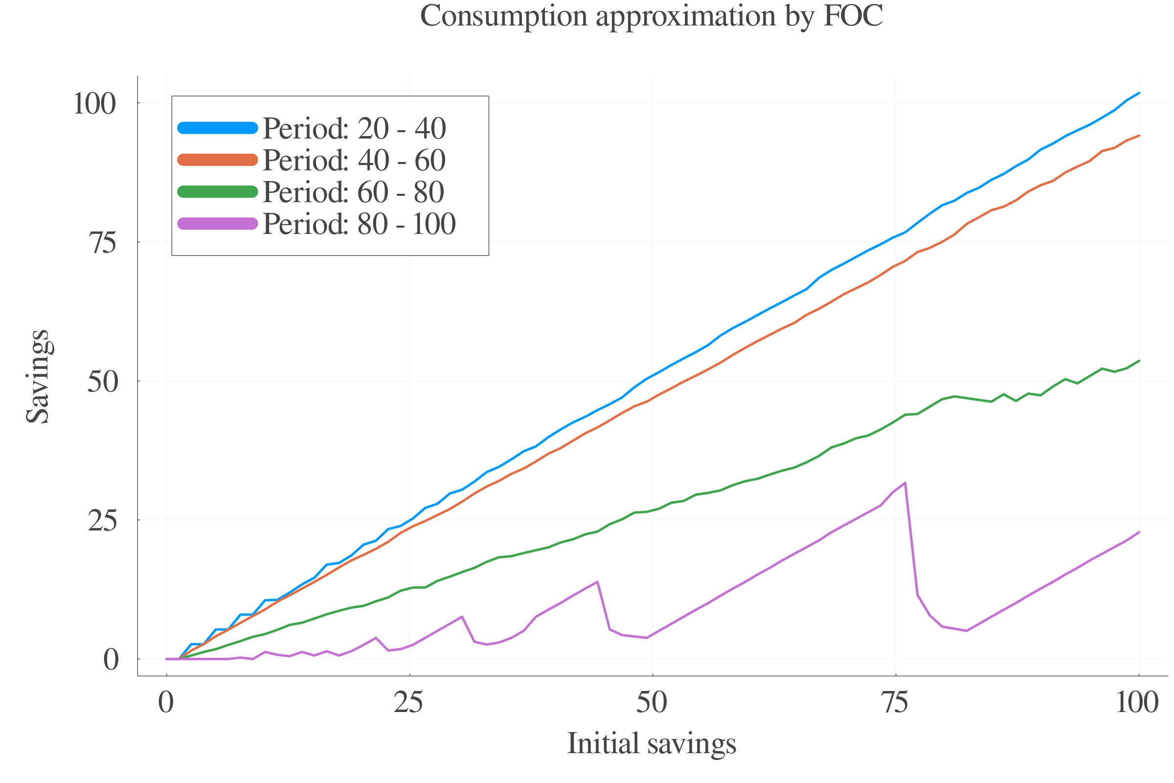
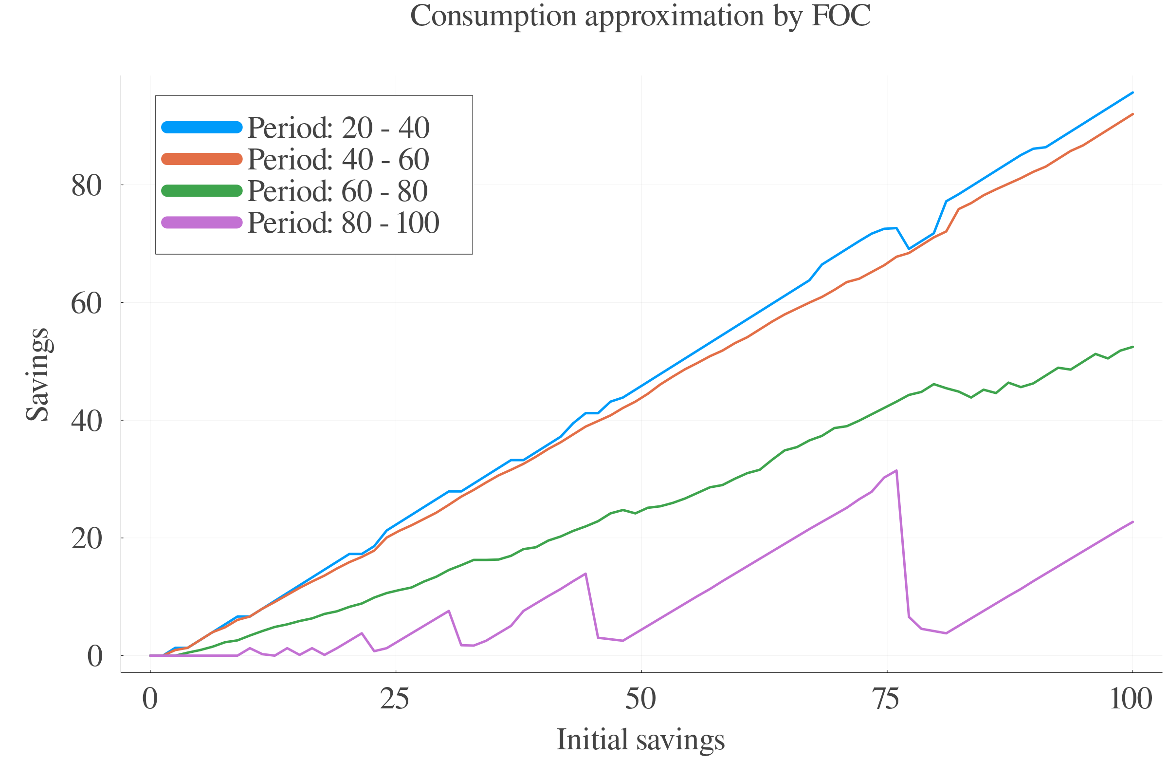
This is a transcendental equation of form \(x^{\alpha}\cdot b - x\cdot y - c = 0\), which admits a solution if and only if \(-\frac{\varphi}{\rho} \in \mathbb{N}\). This condition seems unrealistic in our context:
Note that if we set \(-\rho\in\mathbb{N}\) and further develop the last equation in the budget constraint binding attempt, we end up with the same condition.
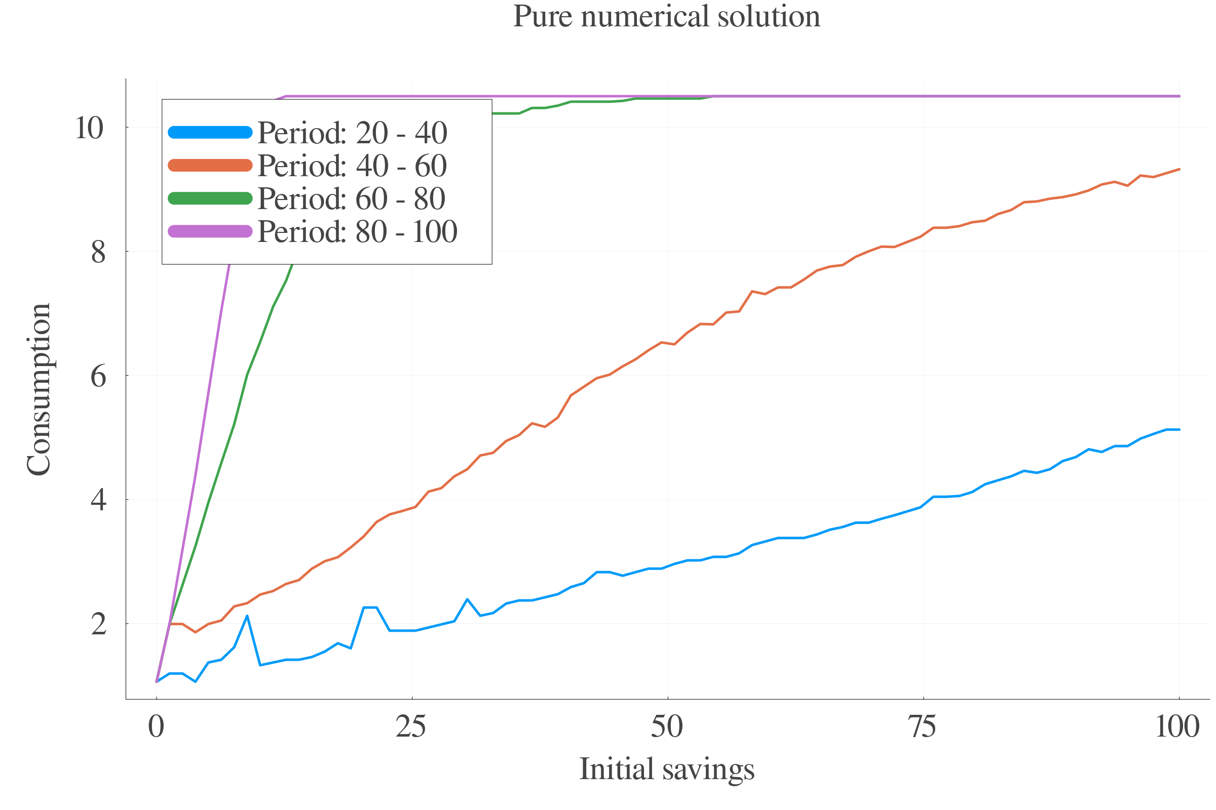
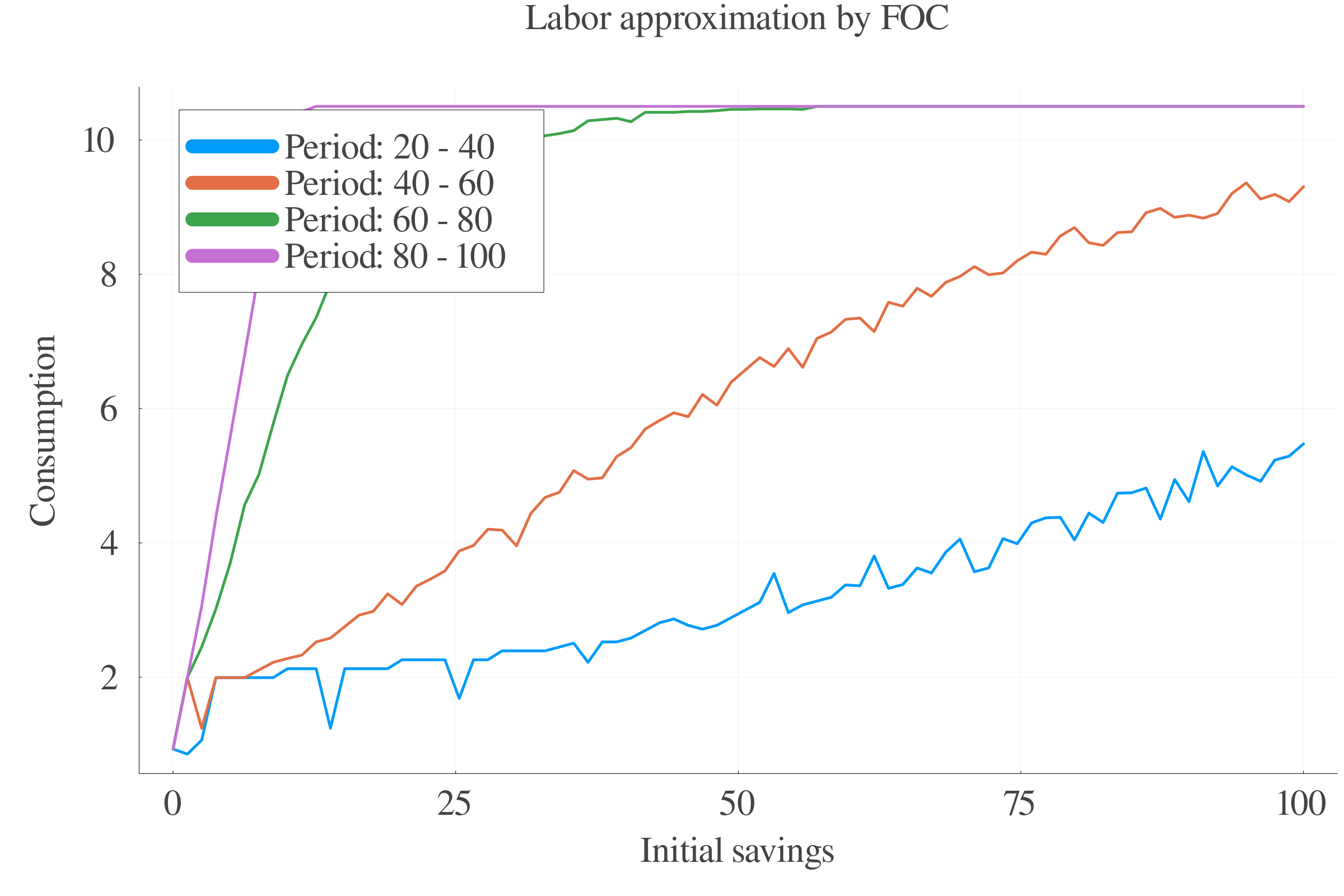
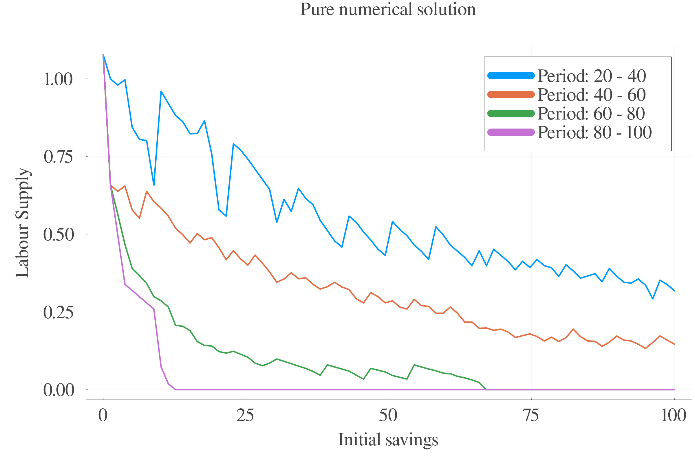
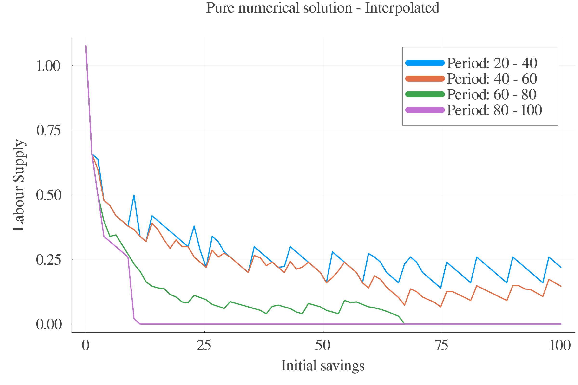
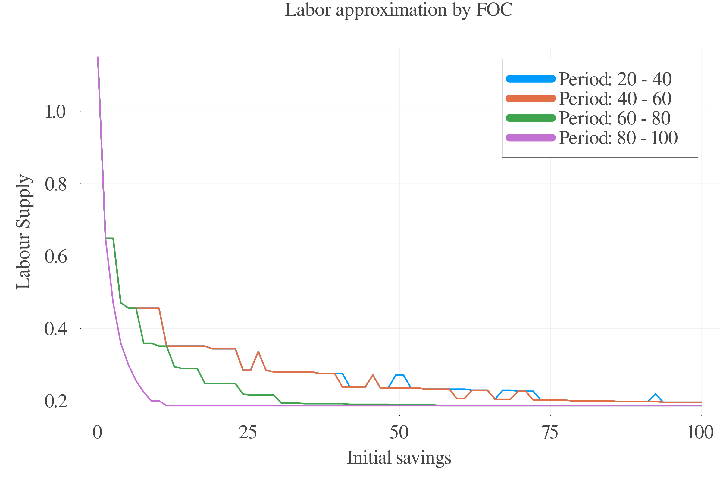
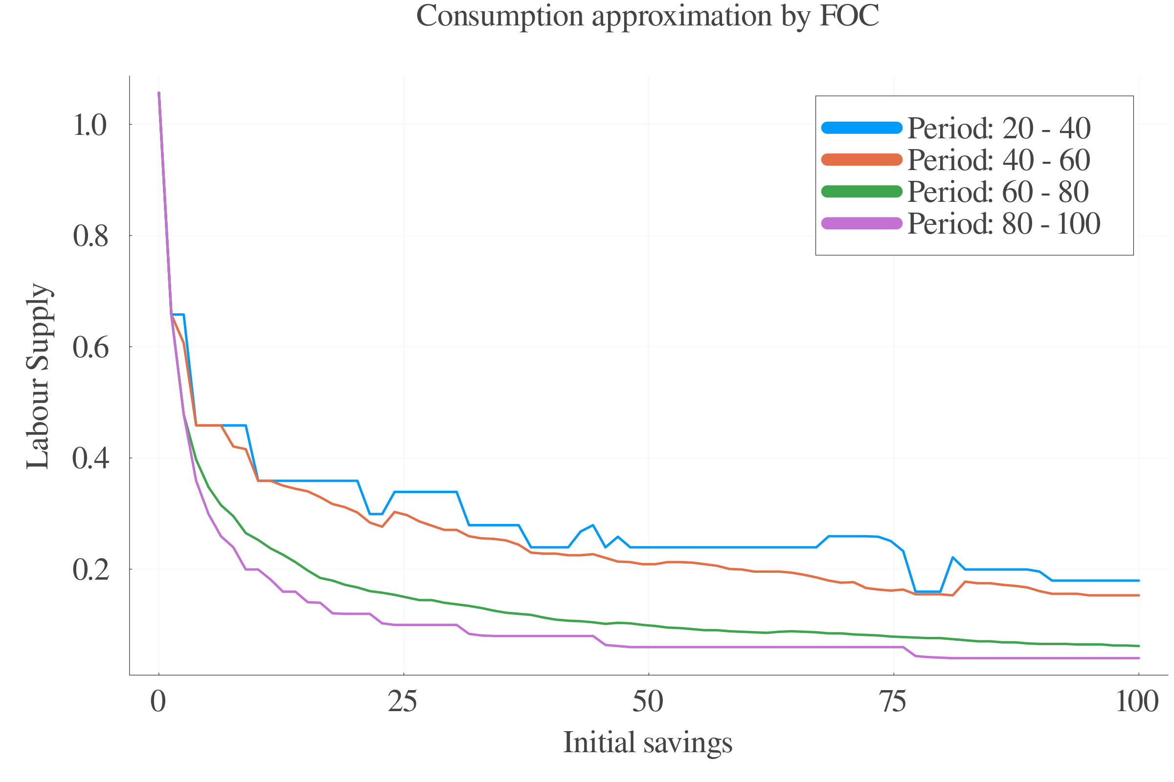
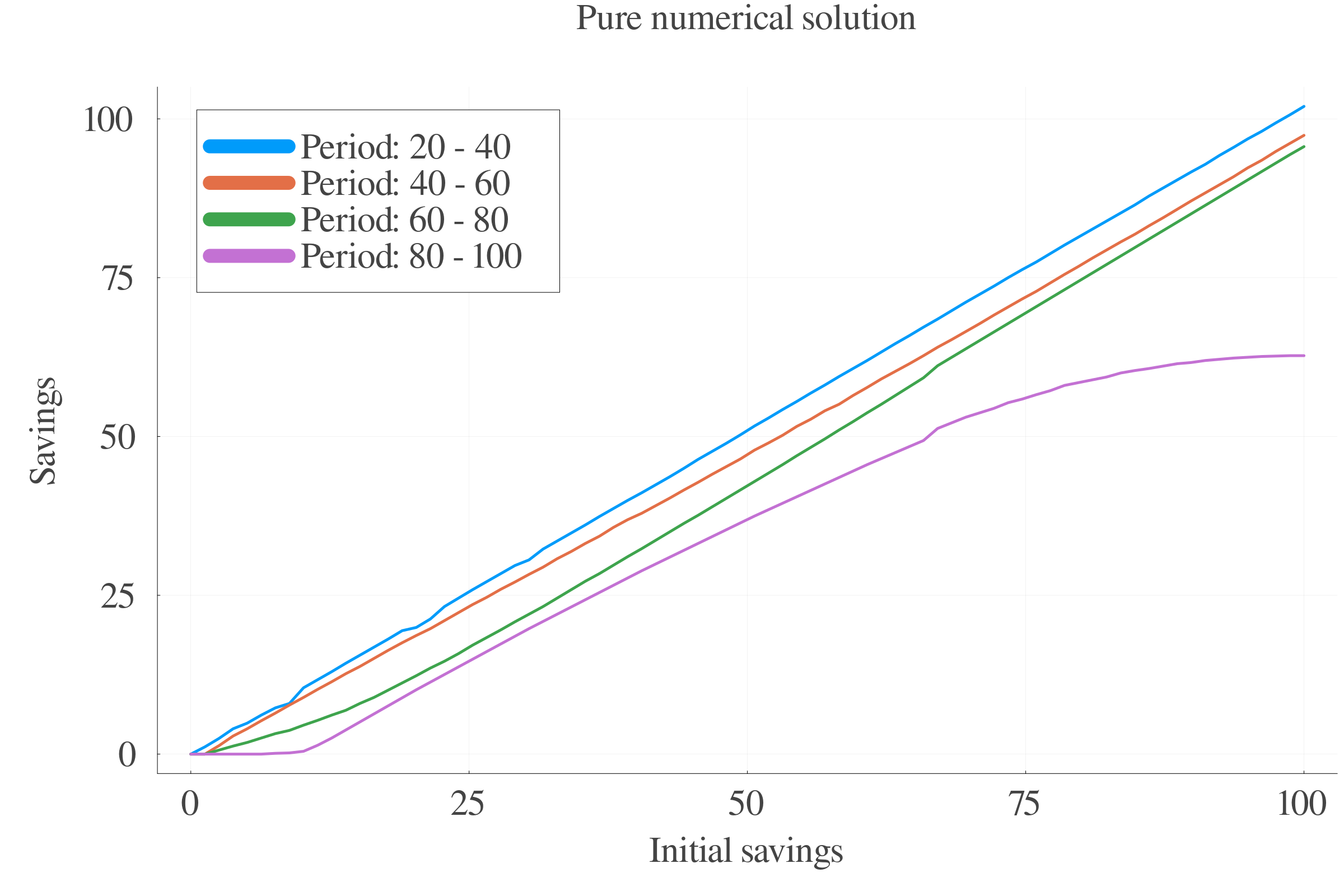
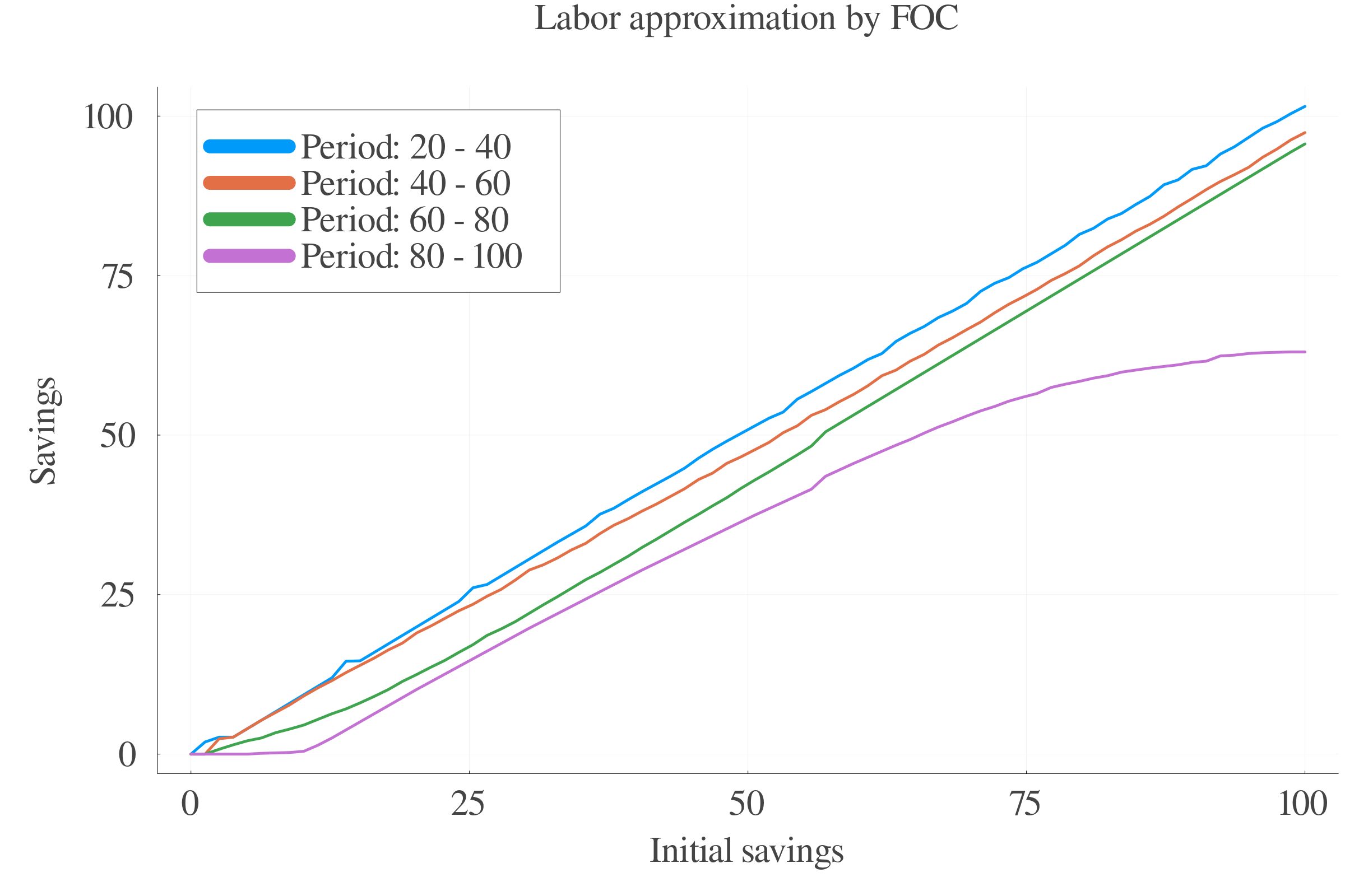
If we try to solve it backwards, we now go to the last period. At the last period, \(s_{t+1} = \underline{s}\) for sure: Since there is no future, the agent will borrow as much as they can, or will at least not save anything more than what is imposed by the constraint.
For simplification, let \(\underline{s}\) be fixed such that: \(\underline{s} = 0\). The new optimality condition is:
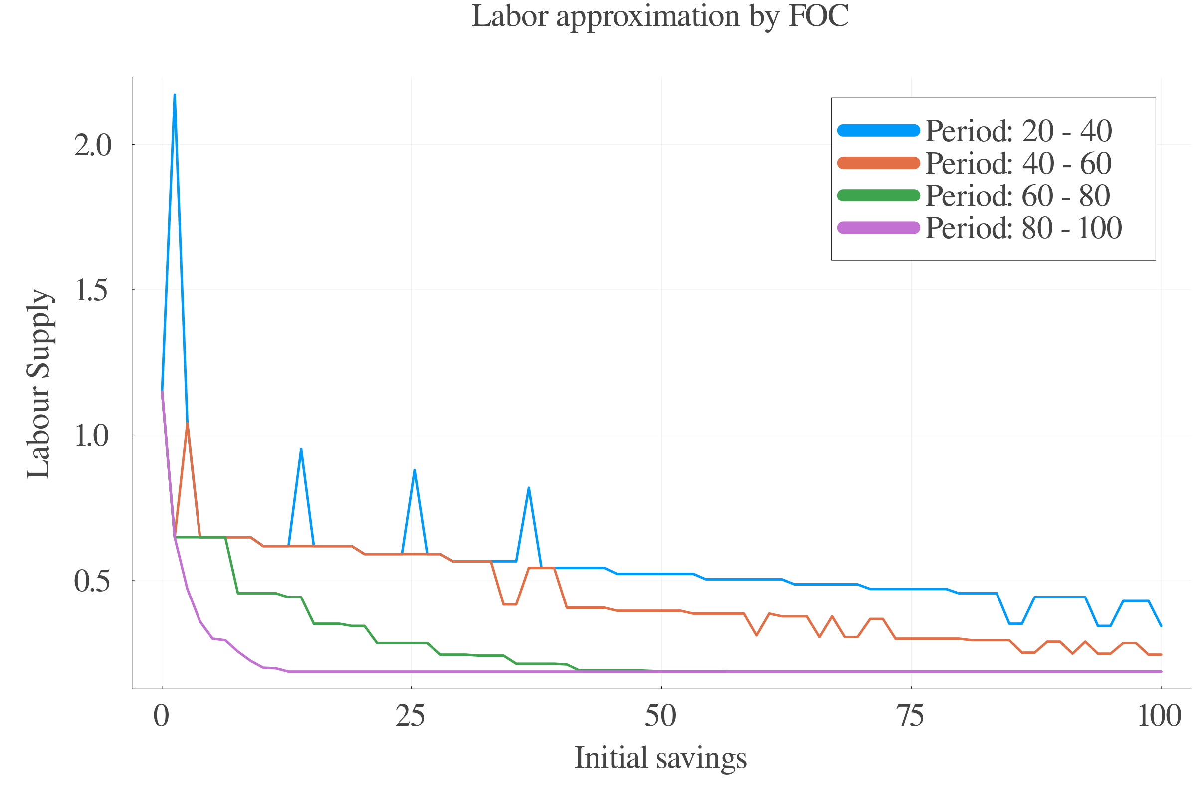
\[\begin{equation}
l_{t}^{\varphi}\cdot \xi_{t} = \left[l_{t}\cdot z_{t} + s_{t}\cdot(1+r_{t})\right]^{-\rho}\cdot z_{t}
\end{equation}\]
Although we simplified the term at the exponential of which we have \(-\rho\), this is still a transcendental equation due to the sum of labor income and income coming from savings of last period, and the problem remain the same.
Go back